Do Marketing Mix Models estimate the true effects of marketing?

We estimate the MMM on our synthetic dataset and compare its estimates to the truth.

Published

August 19, 2026

Introduction

In the previous post, we constructed synthetic data that captures the complexity of a sophisticated retail operation: seasonal patterns, promotional cycles, strategic marketing coordination, and algorithmic bidding. Now we build a Marketing Mix Model, estimate it on this data, and see what it recovers.

We build the model ourselves, from scratch in PyMC. The point is to be transparent and fully understand what happens, and to test the method itself - marketing mix modelling - not a specific implementation of it. We stay deliberately vanilla; readers who want a fuller treatment of MMMs in PyMC can find it in Juan Orduz’ great tutorial.

After building the marketing mix model, we fit it to the synthetic dataset and compare its estimates against the ground truth we built into the data. Does the model identify TV’s 70% carryover? Does it detect the different saturation patterns per channel? And most importantly, are the estimated returns to marketing close to the truth?

Working where the true answers are known is a useful exercise: it lets us see where MMM succeeds and where it struggles, and calibrate our confidence in the methodology before applying it to real data — where nobody will tell us whether we were right.

Setting up the environment

As in the previous post, the plotting functions live in a separate helper file — mmm2_helpers.py — with the same conventions, so the figures of the two posts read as one series.

import numpy as np
import pandas as pd
import xarray as xr
import matplotlib.pyplot as plt
import arviz as az

import pymc as pm
import pytensor.tensor as pt

plt.rcParams.update({
    'axes.spines.top': False, 'axes.spines.right': False,
    'axes.grid': True, 'grid.color': '0.92', 'grid.linewidth': 0.6,
    'axes.axisbelow': True, 'axes.titlelocation': 'left',
    'axes.titleweight': 'normal', 'axes.titlesize': 10.5,
})

np.random.seed(42)
print(f"PyMC version: {pm.__version__}")

PyMC version: 5.22.0

from mmm2_helpers import (
    visualize_roas_comparison,
    visualize_fit_and_decomposition,
    visualize_response_curves,
    visualize_specification_ladder,
)

Step 1: Data Preparation

Before we do any modelling, we have to decide what information the model is allowed to see. The synthetic dataset carries a number of ground-truth columns — the true seasonal component, the latent market sentiment, each channel’s true effect — which only exist because we built the data ourselves; a practitioner working with real data has none of them. To make this a fair test, the model therefore receives exactly what a real analyst would have: total sales, weekly spend per channel, and the observed promotional variables, including their measurement error. We also add ‘the calendar’ as a covariate, and allow for seasonality in sales by adding three annual Fourier harmonics (sine/cosine pairs) as control variables. Everything else stays behind the curtain until it is time to evaluate the estimates.

df = pd.read_csv("synthetic_mmm_data.csv")
df.head()

	week	year	week_of_year	total_sales	base_sales	promotional_sales_uplift	marketing_sales_uplift	seasonal_component	quality_factor	base_price_level	...	true_promotional_price_level	observed_promotion_dummy	observed_promotional_price_level	pla_spend	meta_spend	tv_spend	pla_effect	meta_effect	tv_effect	total_marketing_effect
0	1	1	1	2896.414275	2239.520824	0.000000	656.893451	0.000000	0.049671	1.000000	...	1.000000	0.0	0.957247	140.332692	107.281573	10.860439	463.268805	187.421404	6.203243	656.893451
1	2	1	2	3196.504325	2203.448705	0.000000	993.055621	0.054956	0.044423	1.055973	...	1.055973	0.0	0.920645	198.097935	140.401496	10.937305	681.164797	301.302236	10.588588	993.055621
2	3	1	3	5495.854098	2320.906782	2304.538094	870.409222	0.106231	0.055155	1.064591	...	0.638755	1.0	0.582051	144.755790	80.293109	11.577548	596.991585	259.394564	14.023073	870.409222
3	4	1	4	5903.182328	2605.964209	2587.585093	709.633027	0.150513	0.082858	1.022393	...	0.613436	1.0	0.639042	106.615036	65.177337	10.249844	475.591387	218.372803	15.668836	709.633027
4	5	1	5	5439.086606	2489.169213	2471.613818	478.303576	0.185183	0.074032	1.039850	...	0.623910	1.0	0.618529	60.262295	37.307287	11.007290	305.694983	155.355628	17.252965	478.303576

5 rows × 24 columns

# The analyst's information set
original_data = df[['week', 'total_sales', 'pla_spend', 'meta_spend', 'tv_spend',
                    'observed_promotion_dummy', 'observed_promotional_price_level']].copy()
original_data['date'] = (pd.to_datetime('2022-01-01')
                         + pd.to_timedelta((original_data['week'] - 1) * 7, unit='D'))

media_columns = ['pla_spend', 'meta_spend', 'tv_spend']
control_columns = ['observed_promotion_dummy', 'observed_promotional_price_level']

We use xarray (instead of, say, pandas) to store our dataset, since this works very well together with pymc.

# Everything into labelled xarray containers, scaled by column maxima
sales = xr.DataArray(original_data['total_sales'].values, dims='date',
                     coords={'date': original_data['date']})
media = xr.DataArray(original_data[media_columns].values, dims=('date', 'channel'),
                     coords={'date': original_data['date'],
                             'channel': [c.replace('_spend', '') for c in media_columns]})
controls = xr.DataArray(original_data[control_columns].values, dims=('date', 'control'),
                        coords={'date': original_data['date'], 'control': control_columns})

# for seasonality: three annual harmonics
t = np.arange(len(original_data))
fourier = xr.DataArray(
    np.column_stack([f(2 * np.pi * k * t / 52) for k in (1, 2, 3)
                     for f in (np.sin, np.cos)]),
    dims=('date', 'fourier'),
    coords={'date': original_data['date'],
            'fourier': [f'{f}_{k}' for k in (1, 2, 3) for f in ('sin', 'cos')]})

Scaling

We scale our data before estimation purely for numerical reasons. This is a bit of a technical detail, so feel free to skip this section if you’re not interested.

Right now, note that the scales of different variables and parameters differ by magnitudes:

The values of the sales columns are in the thousands, while saturated adstock is between 0 and 1 for a each channel in a given week.
Consequently, the parameters for \(\lambda\) are in the neighbourhood of 0.01-0.001, while for \(\beta\) they are in the neighbourhood of 100-1000.

This can make it cumbersome (or slow) for the sampler of our Bayesian model. Bringing the variables onto the same scale fixes it.

We divide each series by its historical maximum — what sklearn ships as MaxAbsScaler. This preserves the zero (EUR 0 of unscaled marketing spend will also be EUR 0 of scaled marketing spend), which is important for our model. Dividing by the maximum also keeps the interpretation simple: a scaled spend of 1.0 means “the biggest week we have ever had”, and a scaled spend of 0.5 is half of that.

What scaling costs us is bookkeeping: the model will estimate \(\lambda\) and \(\beta\) in units that depend on the scale of sales and marketing spends, so the raw posteriors are not directly comparable to the data-generating values. Anything that later wants to compare against these posteriors, or to combine with them, has to live on the same scale: this applies to the ground-truth conversion further down this post, and to the geo-test calibration in the next one. We therefore keep track of how we have scaled the variables in a dictionary.

scale_factors = {'total_sales': float(sales.max())}
for col in media_columns + control_columns:
    scale_factors[col] = float(original_data[col].max())

sales_scaled = sales / scale_factors['total_sales']
media_scaled = media / media.max('date')
controls_scaled = controls / controls.max('date')

scale_factors

{'total_sales': 6034.659108756032,
 'pla_spend': 213.73883549513877,
 'meta_spend': 196.75400644639487,
 'tv_spend': 166.88815861711302,
 'observed_promotion_dummy': 1.0,
 'observed_promotional_price_level': 1.2700878252326602}

Lagged spends: setting up adstock

Adstock is a weighted sum of current and past spending, with weights determined by the decay parameter \(\alpha\). There are two ways to give a Bayesian model access to it. One is to pre-compute the adstocked series for a grid of \(\alpha\) values; the other, which we use here, is to hand the model the raw ingredients — current spend plus its first \(\ell_{\max} - 1\) lags — and let it compute the weighted sum inside the computation graph. The second approach is what makes \(\alpha\) a genuinely estimated parameter: the sampler can move it continuously, and the adstock recomputes itself.

With the data already in xarray, the lags are one shift away: media_scaled.shift(date=lag) moves each series down by lag weeks, and stacking the shifts along a new lag dimension gives the three-dimensional block — (date, channel, lag) — that the model will contract against its decay weights. The names are not mere decoration: they let us write the model with broadcasting instead of loops, and they make every posterior object downstream self-describing: trace.posterior["adstock_alpha"].sel(channels="pla") reads like the question it answers.

Two small decisions hide in this cell. First, \(\ell_{\max} = 6\): with normalised geometric weights, six lags carry over 98% of the total weight at \(\alpha = 0.5\), and 88% at \(\alpha = 0.7\), our TV truth — a reasonable truncation, and the same one used when the data were generated, so truncation itself introduces no misspecification here. Second, fill_value=0.0 backfills the lags of the first five weeks with zeros, quietly assuming the company spent nothing before week 1. Over 156 weeks this touches about 3% of the sample and seems harmless.

l_max = 6   # six weeks of adstock memory

media_lagged = xr.concat(
    [media_scaled.shift(date=lag, fill_value=0.0) for lag in range(l_max)],
    dim=pd.Index(range(l_max), name='lag'),
).transpose('date', 'channel', 'lag')

data = xr.Dataset({
    'sales': sales_scaled,
    'media': media_lagged,
    'controls': controls_scaled,
    'fourier_terms': fourier
})
data

# PyMC works on dense arrays; extract them once, keeping the names as coords
media_data = data.media.values          # (periods, channels, lags)
y_observed = data.sales.values
controls_data = data.controls.values    # (periods, controls)
fourier_data = data.fourier_terms.values

n_periods, n_channels, n_lags = media_data.shape
n_controls = len(control_columns)
n_fourier = fourier_data.shape[1]
print(f"Data dimensions: {n_periods} periods, {n_channels} channels, "
      f"{n_lags} lags, {n_controls} controls, {n_fourier} seasonal terms")

Data dimensions: 156 periods, 3 channels, 6 lags, 2 controls, 6 seasonal terms

Step 2: Build and estimate the model

Defining the model

The data is now in shape - scaled, lagged, labelled. Next, we define the model and read through it to understand what it does.

coords = {
    'periods': range(n_periods),
    'channels': data.coords['channel'].values,   # ['pla', 'meta', 'tv']
    'lags': range(n_lags),
    'controls': control_columns,
    'fourier': data.coords['fourier'].values
}

with pm.Model(coords=coords) as mmm_model:

    # Priors
    adstock_alpha = pm.Beta("adstock_alpha", alpha=2, beta=1, dims="channels")
    saturation_lambda = pm.Gamma("saturation_lambda", alpha=2, beta=1, dims="channels")
    beta_media = pm.Normal("beta_media", mu=0, sigma=0.5, dims="channels")
    beta_controls = pm.Normal("beta_controls", mu=0, sigma=0.3, dims="controls")
    beta_fourier = pm.Normal("beta_fourier", mu=0, sigma=0.2, dims="fourier")
    intercept = pm.Normal("intercept", mu=0.5, sigma=0.2)
    sigma = pm.HalfNormal("sigma", sigma=0.1)

    # === MARKETING TRANSFORMATIONS: raw spend -> sales impact ===

    # Step 1: carryover (adstock). Geometric decay weights [1, a, a^2, ...]
    lag_indices = pt.arange(n_lags)
    decay_weights = pt.power(
        adstock_alpha.dimshuffle(0, 'x'),   # (channels, 1)
        lag_indices.dimshuffle('x', 0)      # (1, lags)
    )                                        # -> (channels, lags)

    # Normalise so carryover redistributes effect without creating it
    normalized_weights = decay_weights / pt.sum(decay_weights, axis=1, keepdims=True)

    media_adstocked = pm.Deterministic(
        "media_adstocked",
        pt.sum(media_data * normalized_weights.dimshuffle('x', 0, 1), axis=2),
        dims=("periods", "channels")
    )

    # Step 2: diminishing returns (saturation)
    media_saturated = pm.Deterministic(
        "media_saturated",
        (1 - pt.exp(-saturation_lambda * media_adstocked)) /
        (1 + pt.exp(-saturation_lambda * media_adstocked)),
        dims=("periods", "channels")
    )

    # Step 3: scale to sales impact
    media_contribution = pm.Deterministic(
        "media_contribution",
        pt.sum(media_saturated * beta_media, axis=1),
        dims="periods"
    )

    # === CONTROL EFFECTS ===
    control_contribution = pm.Deterministic(
        "control_contribution",
        pt.sum(controls_data * beta_controls, axis=1),
        dims="periods"
    )

    # === SEASONALITY ===
    seasonal_contribution = pm.Deterministic(
        "seasonal_contribution",
        pt.sum(fourier_data * beta_fourier, axis=1),
        dims="periods"
    )

    # === MEAN AND LIKELIHOOD ===
    mu = pm.Deterministic("mu", intercept + media_contribution
                          + control_contribution + seasonal_contribution,
                          dims="periods")
    sales_obs = pm.Normal("sales_obs", mu=mu, sigma=sigma,
                          observed=y_observed, dims="periods")

Reading the model

The block reads as the generator from the previous post run in reverse. Every operation the generator performed — lag, decay, saturate, scale, sum — appears again, in the same order and the same functional form. What has changed is the direction of the numbers. The generator was handed marketing spends and the parameters to translate them into sales (i.e. for TV \(\alpha = 0.7\), \(\lambda = 0.006\), \(\beta = 560\)). This model is handed marketing spends and sales and asked what the parameters \(\alpha, \lambda, \beta\) must have been. That inversion is the entire content of this section: the three constants per channel that the previous post typed into CHANNEL_CONFIGS have become random variables with priors, which we are looking to recover.

Follow one channel through the model.

A channel’s adstock in a given week is a function of its spend in this week, the five previous weeks, and the parameter \(\alpha\). We calculate this in step 1. The decay weights \([1, \alpha, \alpha^2, \dots]\) are computed from adstock_alpha inside the computation graph, normalised to sum to one, and contracted against the lag dimension; when the sampler proposes a new \(\alpha\), the weights and everything downstream recompute. The result is the channel’s adstock in each week.
Saturation then converts adstock into saturated adstock, a number between zero and one per week; and \(\beta\) converts that fraction into incremental sales due to that channel’s marketing.
A week’s total sales are then just a sum: the incremental sales of the three channels, plus everything that is not marketing — the intercept, the control variables, and the seasonal curve traced by the Fourier terms — plus some random noise (entering through the likelihood).

One asymmetry in that sum deserves a sentence. The marketing side of the equation is exactly the generator’s — same lags, same adstock, same saturation. The non-marketing side is not: the true baseline is multiplicative in its components, while intercept and controls, and seasonal terms enter linearly here. Whatever goes wrong with the media estimates, then, cannot be blamed on functional form; the open question is whether the data contain the information, which is the question the experiment was built to isolate.

pm.model_to_graphviz(mmm_model)

The same model, drawn

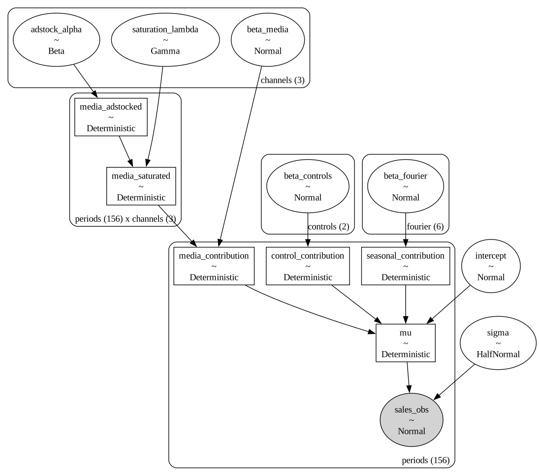
The graphviz output above is this walk-through as a picture, in the plate notation used for Bayesian models, and having read the walk-through you can read the diagram in thirty seconds. The ellipses are the random variables: unfilled for the parameters we estimate, each labelled with its prior, and shaded for sales_obs — shading marks what the model conditions on. The plain rectangles are the deterministic way-stations from the walk-through: adstock, saturated adstock, marketing contributions, mu. The rounded boxes — the plates — express repetition, and they encode the model’s assumptions more compactly than the code does: adstock_alpha, saturation_lambda, and beta_media sit inside the channels (3) plate, so each channel gets its own carryover, its own curve, its own ceiling; beta_fourier sits in its own fourier (6) plate — six coefficients jointly shaping one smooth yearly curve; intercept and sigma sit outside every plate, so all weeks share one baseline and one noise level. (The raw spend and control arrays appear nowhere — they entered as plain numpy constants, and the graph shows only what is uncertain or derived.)

Priors, briefly

The priors are weakly informative and, for the most part, not where the action is; the interesting question is downstream, whether the estimated returns match the truth. Three choices are still worth naming. The carryover prior, Beta(2, 1), leans toward high carryover — its mean of two-thirds is a prior half-life of about 1.7 weeks — and this is a deliberate, debatable choice: pymc-marketing ships Beta(1, 3), mean one-quarter, as its default, and the companion paper re-runs everything under those priors to confirm nothing hinges on it. The media coefficients are centred at zero and not constrained positive, so the data remain free to conclude that a channel does nothing, or worse. And the remaining priors simply live comfortably in scaled units, where everything is a fraction of the best week ever: an intercept around 0.5 because baseline carries most of sales, seasonal coefficients at Normal(0, 0.2), noise around a tenth of the maximum, and a saturation prior whose mean of 2 puts the half-saturation spend near half of the biggest spending week — the truth for PLA, for comparison, works out to about 1.7 in these units.

Estimating the model

Sampling uses NUTS, the default gradient-based sampler: four chains of 1,000 draws after 1,000 tuning steps, with target_accept = 0.95.

with mmm_model:
    trace = pm.sample(
        draws=1000,
        tune=1000,
        chains=4,
        target_accept=0.95,
        random_seed=42,
        return_inferencedata=True
    )

Initializing NUTS using jitter+adapt_diag...
Multiprocess sampling (4 chains in 4 jobs)
NUTS: [adstock_alpha, saturation_lambda, beta_media, beta_controls, beta_fourier, intercept, sigma]

Sampling 4 chains for 1_000 tune and 1_000 draw iterations (4_000 + 4_000 draws total) took 13 seconds.

az.plot_trace(trace, var_names=["adstock_alpha", "saturation_lambda", "beta_media",
                                "beta_controls", "intercept", "sigma"]);

az.summary(trace, var_names=["adstock_alpha", "saturation_lambda",
                             "beta_media", "beta_controls"])

	mean	sd	hdi_3%	hdi_97%	mcse_mean	mcse_sd	ess_bulk	ess_tail	r_hat
adstock_alpha[pla]	0.493	0.091	0.316	0.649	0.002	0.001	1775.0	2986.0	1.0
adstock_alpha[meta]	0.484	0.323	0.023	0.964	0.010	0.002	1337.0	2488.0	1.0
adstock_alpha[tv]	0.660	0.246	0.216	1.000	0.004	0.003	2853.0	1655.0	1.0
saturation_lambda[pla]	1.421	0.567	0.556	2.528	0.010	0.012	2575.0	2443.0	1.0
saturation_lambda[meta]	1.440	1.133	0.048	3.319	0.021	0.039	2663.0	2540.0	1.0
saturation_lambda[tv]	1.282	1.152	0.005	3.410	0.020	0.027	1957.0	1824.0	1.0
beta_media[pla]	0.664	0.239	0.268	1.119	0.005	0.005	2332.0	2062.0	1.0
beta_media[meta]	-0.143	0.298	-0.679	0.498	0.007	0.007	1611.0	1636.0	1.0
beta_media[tv]	0.005	0.176	-0.301	0.401	0.006	0.009	1076.0	1407.0	1.0
beta_controls[observed_promotion_dummy]	0.037	0.011	0.017	0.058	0.000	0.000	4646.0	2984.0	1.0
beta_controls[observed_promotional_price_level]	-0.627	0.042	-0.704	-0.546	0.001	0.001	2659.0	2859.0	1.0

Reading the diagnostics

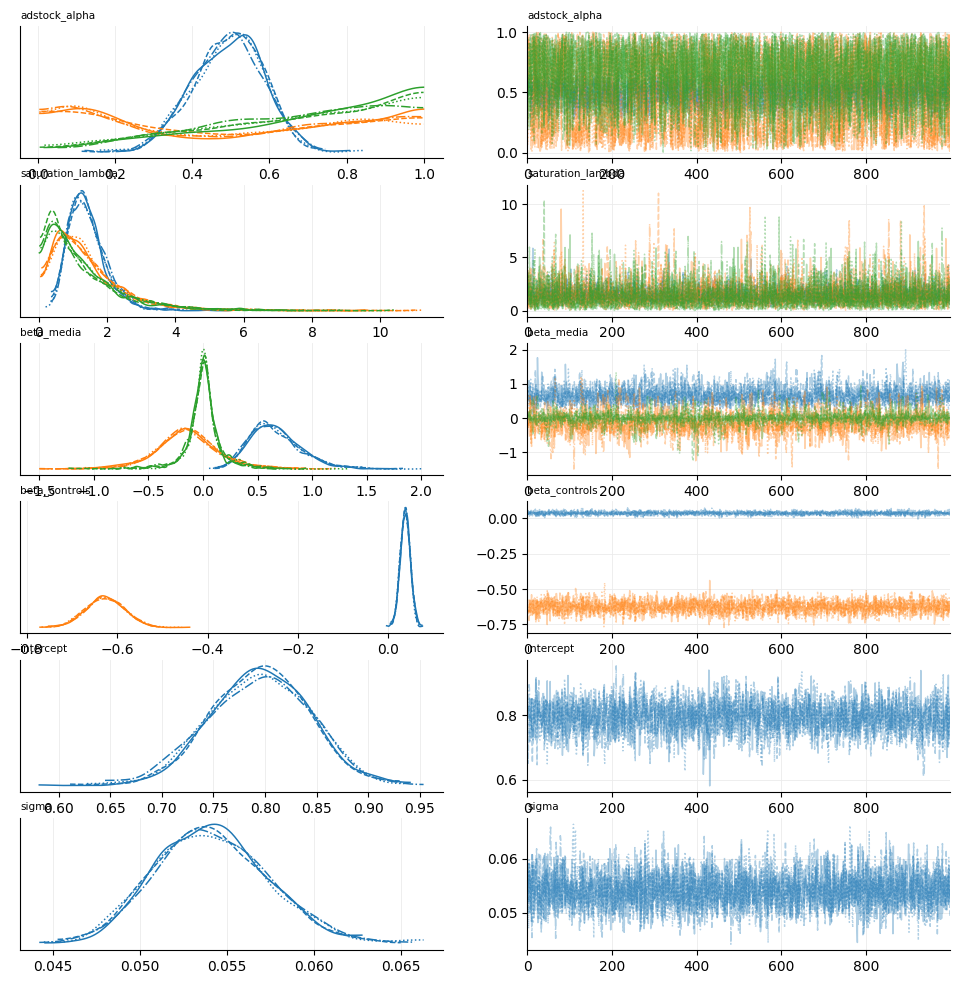
The trace plots and the summary table answer one question only: did the sampler manage to characterise the posterior? In the trace plots, healthy chains look like dense, stationary noise with all four chains overplotting each other; trends, drifts, or chains exploring different regions signal trouble. In the table, r_hat compares within-chain to between-chain variance and should sit below 1.01, while ess_bulk and ess_tail report how many effectively independent draws we obtained — enough in our case.

All of these checks pass here. Still, it is worth being precise about what that does and does not establish, because the distinction is the theme of this post: convergence diagnostics validate the computation, not the inference. A sampler can converge impeccably to a posterior that is confidently wrong, and we are about to watch it do exactly that.

A note on units before we compare anything

This is the bill for the scaling in Step 1 coming due. The model was estimated on scaled data — each series divided by its maximum — so the posterior parameters live in scaled units, and the scale_factors dictionary we kept is what lets us translate. The conversion differs by parameter:¹

Adstock \(\alpha\) is scale-free. Rescaling spend does not change the shape of the carryover decay, so the posterior for adstock_alpha is directly comparable to the true values (0.2, 0.4, 0.7).
Saturation \(\lambda\) scales with spend. The model sees \(x / \max(x)\), so it must estimate \(\lambda_{\text{scaled}} = \lambda_{\text{true}} \times \max(x)\) to reproduce the same curve.
The effect coefficient \(\beta\) scales with sales. The model predicts \(y / \max(y)\), so \(\beta_{\text{scaled}} = \beta_{\text{true}} / \max(y)\).

This has a practical consequence- for \(\alpha\), we can directly compare the estimated parameter to that of the data generating process; for \(\lambda\) and \(\beta\) we must rescale the parameters to make them comparable.

One further note — for \(\lambda\) and \(\beta\), individual parameters are weakly identified. A “wrong” \(\lambda\) paired with a compensating \(\beta\) can produce a nearly identical response curve over the observed spend range. What the data pin down is their joint implication — the incremental sales attributed to each channel, and hence the ROAS. We keep this in mind when reading the table below and hence focus on the response curve and the ROAS it implies.

# Ground-truth parameters from the data-generating notebook, and their scaled equivalents
TRUE_CONFIGS = {
    'pla_spend':  {'alpha': 0.2, 'lambda': 0.008, 'beta': 1100},
    'meta_spend': {'alpha': 0.4, 'lambda': 0.010, 'beta': 600},
    'tv_spend':   {'alpha': 0.7, 'lambda': 0.006, 'beta': 560},
}

rows = []
y_max = scale_factors['total_sales']
for ch_idx, ch in enumerate(media_columns):
    cfg = TRUE_CONFIGS[ch]
    x_max = scale_factors[ch]
    post_a = trace.posterior['adstock_alpha'].values[:, :, ch_idx].flatten()
    post_l = trace.posterior['saturation_lambda'].values[:, :, ch_idx].flatten()
    post_b = trace.posterior['beta_media'].values[:, :, ch_idx].flatten()
    rows.append({
        'channel': ch.replace('_spend', '').upper(),
        'alpha_true': cfg['alpha'],
        'alpha_est': f"{post_a.mean():.2f} [{np.percentile(post_a, 5):.2f}, {np.percentile(post_a, 95):.2f}]",
        'lambda_scaled_true': round(cfg['lambda'] * x_max, 2),
        'lambda_est': f"{post_l.mean():.2f} [{np.percentile(post_l, 5):.2f}, {np.percentile(post_l, 95):.2f}]",
        'beta_scaled_true': round(cfg['beta'] / y_max, 3),
        'beta_est': f"{post_b.mean():.3f} [{np.percentile(post_b, 5):.3f}, {np.percentile(post_b, 95):.3f}]",
    })

param_recovery = pd.DataFrame(rows).set_index('channel')
param_recovery

	alpha_true	alpha_est	lambda_scaled_true	lambda_est	beta_scaled_true	beta_est
channel
PLA	0.2	0.49 [0.34, 0.63]	1.71	1.42 [0.68, 2.48]	0.182	0.664 [0.332, 1.094]
META	0.4	0.48 [0.05, 0.96]	1.97	1.44 [0.27, 3.53]	0.099	-0.143 [-0.616, 0.356]
TV	0.7	0.66 [0.20, 0.98]	1.00	1.28 [0.16, 3.59]	0.093	0.005 [-0.247, 0.288]

The table shows the estimated parameters and true parameters (rescaled, to account for the fact we rescaled marketing spends and sales) — so they are now directly comparable. Throughout, brackets are 90% credible intervals. The verdict, following what we established above: judge the model not on its parameters but on what they jointly imply. That is the comparison we turn to now.

Step 3: Examining the estimates

The quantity a budget owner cares about is incremental sales per euro spent (sometimes called ROAS - return on ad spend). Our model has estimated the incremental sales that each marketing channel generated; but we also know the true incremental sales, since we build the synthetic dataset ourselves. Marketing spends are known, so calculating both estimated ROAS and true ROAS for each channel is easy: incremental sales divided by marketing spend.

Two remarks before the code. The return on ad spend we calculate here is an average return, not a marginal one, and under saturation the two differ: the average grades the spending history (i.e. total incremental sales divided by total marketing spend), the marginal tell us the return on the next euro. And we compute returns per posterior draw, so the ROAS arrives as a full distribution with the correlations between \(\lambda\) and \(\beta\) propagated rather than plugged in at their means.

# === ROAS ===
# Contribution over spend, per posterior draw, on both sides of the comparison.

def roas_by_channel(trace):
    """Posterior ROAS per channel, from the trace's stored contributions."""
    incremental = (trace.posterior['media_saturated']
                   * trace.posterior['beta_media']).sum('periods')   # (chain, draw, channels)
    spend = xr.DataArray([original_data[ch].sum() for ch in media_columns],
                         dims='channels', coords={'channels': incremental['channels']})
    return incremental * y_max / spend

roas = roas_by_channel(trace)

# The ground truth, straight from the data-generating process
true_roas = {ch: df[ch.replace('_spend', '_effect')].sum() / df[ch].sum()
             for ch in media_columns}

summ = az.summary(roas.to_dataset(name='roas'), hdi_prob=0.90, kind='stats')
comparison = pd.DataFrame({
    'True_ROAS': [true_roas[ch] for ch in media_columns],
    'Est_ROAS': summ['mean'].values,
    'HDI90_Lower': summ['hdi_5%'].values,
    'HDI90_Upper': summ['hdi_95%'].values,
}, index=['PLA', 'Meta', 'TV'])
comparison['In_HDI90'] = comparison['True_ROAS'].between(
    comparison['HDI90_Lower'], comparison['HDI90_Upper'])
comparison.round(2)

	True_ROAS	Est_ROAS	HDI90_Lower	HDI90_Upper	In_HDI90
PLA	4.20	11.52	6.92	15.70	False
Meta	2.90	-2.19	-8.72	5.09	True
TV	1.56	0.11	-2.70	2.41	True

visualize_roas_comparison(roas, true_roas, media_columns)

What the ROAS comparison shows

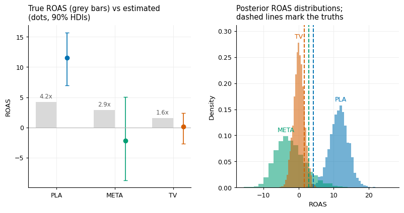
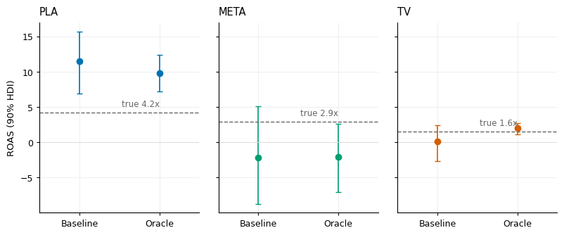
The estimates fail in two different ways, and the difference is instructive. Estimates for PLA — the algorithmically managed channel — are confidently wrong: a true return of 4.2 is estimated at 11.5, with a 90% interval of [6.9, 15.7] that excludes the truth by a substantial margin. The model has to place the sales somewhere; because PLA’s spend moves with the sales it did not cause, PLA is where the sales go. Meta and TV fail in the opposite direction: their intervals do contain the truths — the table dutifully reports True — but only because they are too wide to say anything. Meta’s spans −8.7 to 5.1 around a truth of 2.9, with a point estimate that is actually negative; TV’s spans −2.7 to 2.4 around 1.6. An interval that cannot distinguish “this channel returns three euros per euro” from “this channel destroys value” has not identified anything; it has merely declined to commit.

Step 4: Where did the sales go? Fit and decomposition

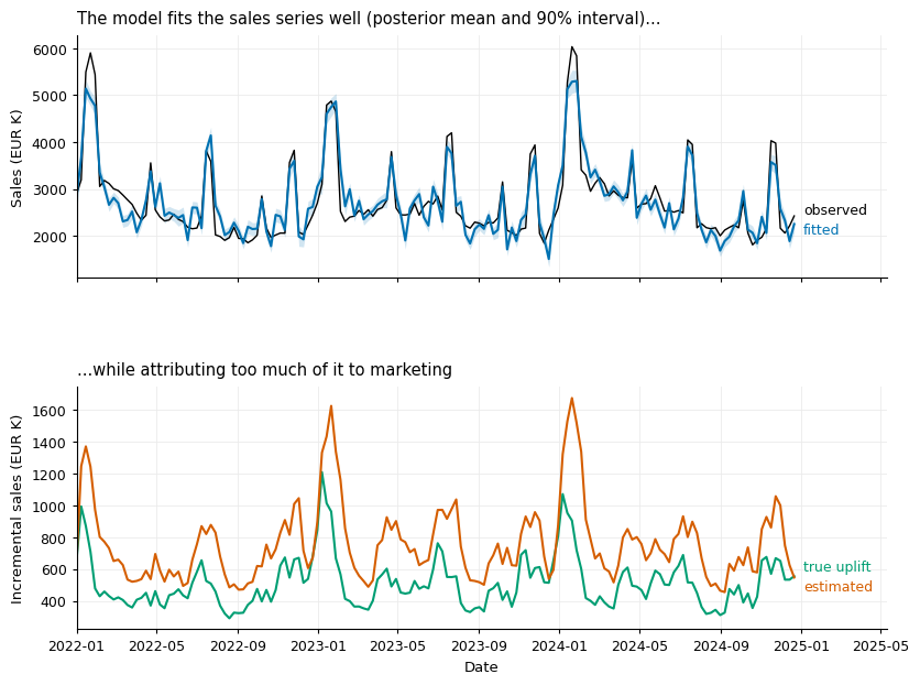
Predictive checks would tell us the model fits well. The interesting question is how it fits well — which components carry the variation. We compare the model’s fitted sales against the observed series, and its estimated marketing contribution against the true one.

visualize_fit_and_decomposition(
    trace,
    dates=original_data['date'],
    observed_sales=original_data['total_sales'],
    true_uplift=df['marketing_sales_uplift'],
    y_max=y_max,
)

True marketing share of sales:      18.7%
Estimated marketing share of sales: 27.7%

The two panels tell the story of this post in miniature. Predictive fit is good — the model tracks seasonality, promotions, everything. But it achieves that fit partly by routing baseline variation through the media variables, because the media variables move with the baseline: the bidding algorithm raised PLA spend whenever recent sales were strong, and budgets grew after good quarters. The model ends up with a good fit built on a wrong decomposition — and this is precisely the difference between prediction and causal inference, drawn here by the data itself.

Response curves

For budget decisions, the object of interest is the response curve — incremental sales as a function of weekly spend. Because the adstock weights are normalised, a constant weekly spend of \(x\) produces an adstocked value of \(x\), so the steady-state weekly response is simply \(\beta \cdot g(\lambda x)\). We can draw the posterior curves against the truth.

def logistic_saturation_np(x, lam):
    """Diminishing returns — the same functional form as inside the model."""
    return (1 - np.exp(-lam * x)) / (1 + np.exp(-lam * x))

visualize_response_curves(
    trace,
    media_columns=media_columns,
    spend_data=original_data,
    scale_factors=scale_factors,
    true_configs=TRUE_CONFIGS,
    saturation_fn=logistic_saturation_np,
)

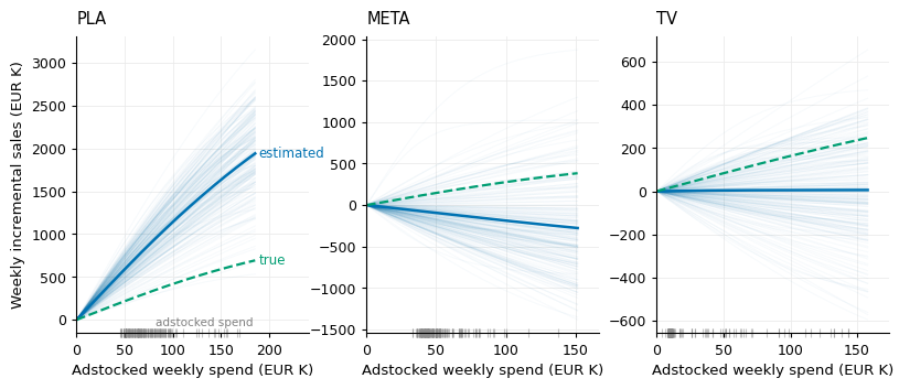
The ticks mark each channel’s actual adstocked spend in our weekly data (note that adstock is also an estimate, since it depends on \(\alpha\); I’ve calculated the adstock displayed here using the mean posterior alpha for each channel). The adstocked spends show the variation that the model learns from when trying to estimate each channel’s saturation; everything outside it is extrapolation. Note that adstocked spends are concentrated in relatively narrow ranges, where (true) saturation curves are relatively flat. This means estimating the curvature of the saturation curves is extremely difficult. As we see from the estimates, the model cannot tell saturation from a straight line, so what it really pins down per channel is only a slope.

Step 5: The oracle test

Where does this leave an analyst? The model is honestly specified — the calendar controlled, the promotional variables in — and it is still confidently wrong about PLA. The standard advice at this point is as old as regression: add better controls. Find covariates that track demand — category indices, competitor activity, weather, search trends — and the confounding will be absorbed. It is reasonable advice, and it is also open-ended: in the field, one can always believe that the next covariate would have fixed it, because nothing ever tells you that you have controlled for enough.

Here we can do what no analyst can: skip to the end of that road. We built the demand, so we can hand the model demand itself — the true seasonal component, the true quality drift, the true market sentiment, and the true promotional state, free of measurement error. These are not better proxies; they are the quantities the proxies try to approximate, covariates no practitioner will ever possess. This “oracle” specification is therefore not a realistic model but an upper bound on the entire better-controls programme: whatever any achievable set of covariates could absorb, these absorb more. The test is correspondingly clean. If the oracle recovers PLA, the baseline’s failure was omitted variables, and the practical problem is merely data quality. If even the oracle fails, no controls can succeed, and the problem sits deeper.

To keep the comparison honest, the oracle is the same model with the information swapped: build_mmm below is the model block from Step 2, line for line, with the control matrix passed in as an argument. Two details. The Fourier terms are switched off, because the oracle receives the true seasonal path directly — estimating harmonics to approximate a curve the model has already been handed would be redundant. And the controls get generous Normal(0, 2) priors, so the priors cannot be accused of holding perfect covariates back.

def build_mmm(controls_data, control_names, fourier_data=None, control_sigma=0.3):
    """The model of Step 2, verbatim, parameterised by its information set."""
    cds = {'periods': range(n_periods),
           'channels': data.coords['channel'].values,
           'lags': range(n_lags),
           'controls': control_names}
    if fourier_data is not None:
        cds['fourier'] = data.coords['fourier'].values
    with pm.Model(coords=cds) as model:
        adstock_alpha = pm.Beta("adstock_alpha", alpha=2, beta=1, dims="channels")
        saturation_lambda = pm.Gamma("saturation_lambda", alpha=2, beta=1, dims="channels")
        beta_media = pm.Normal("beta_media", mu=0, sigma=0.5, dims="channels")
        beta_controls = pm.Normal("beta_controls", mu=0, sigma=control_sigma, dims="controls")
        intercept = pm.Normal("intercept", mu=0.5, sigma=0.2)
        sigma = pm.HalfNormal("sigma", sigma=0.1)

        lag_indices = pt.arange(n_lags)
        decay_weights = pt.power(adstock_alpha.dimshuffle(0, 'x'),
                                 lag_indices.dimshuffle('x', 0))
        normalized_weights = decay_weights / pt.sum(decay_weights, axis=1, keepdims=True)

        media_adstocked = pt.sum(media_data * normalized_weights.dimshuffle('x', 0, 1), axis=2)
        media_saturated = pm.Deterministic(
            "media_saturated",
            (1 - pt.exp(-saturation_lambda * media_adstocked)) /
            (1 + pt.exp(-saturation_lambda * media_adstocked)),
            dims=("periods", "channels"))
        media_contribution = pm.Deterministic(
            "media_contribution", pt.sum(media_saturated * beta_media, axis=1), dims="periods")
        control_contribution = pt.sum(controls_data * beta_controls, axis=1)

        mu = intercept + media_contribution + control_contribution
        if fourier_data is not None:
            beta_fourier = pm.Normal("beta_fourier", mu=0, sigma=0.2, dims="fourier")
            mu = mu + pm.Deterministic(
                "seasonal_contribution",
                pt.sum(fourier_data * beta_fourier, axis=1), dims="periods")

        pm.Normal("sales_obs", mu=pm.Deterministic("mu", mu, dims="periods"),
                  sigma=sigma, observed=y_observed, dims="periods")
    return model

oracle_controls = np.column_stack([
    df['true_promotion_dummy'].values,
    df['true_promotional_price_level'].values,
    df['seasonal_component'].values,
    df['quality_factor'].values,
    df['market_sentiment'].values,
])
oracle_names = ['true_promo_dummy', 'true_price_level',
                'seasonal', 'quality', 'sentiment']

mmm_model_oracle = build_mmm(oracle_controls, oracle_names, fourier_data=None, control_sigma=2.0)
with mmm_model_oracle:
    trace_oracle = pm.sample(
        draws=1000, tune=1000, chains=4, target_accept=0.97,
        random_seed=42, return_inferencedata=True,
    )

Initializing NUTS using jitter+adapt_diag...
Multiprocess sampling (4 chains in 4 jobs)
NUTS: [adstock_alpha, saturation_lambda, beta_media, beta_controls, intercept, sigma]

Sampling 4 chains for 1_000 tune and 1_000 draw iterations (4_000 + 4_000 draws total) took 26 seconds.

roas_oracle = roas_by_channel(trace_oracle)
summ_o = az.summary(roas_oracle.to_dataset(name='roas'), hdi_prob=0.90, kind='stats')

comparison_oracle = pd.DataFrame({
    'True_ROAS': [true_roas[ch] for ch in media_columns],
    'Baseline': comparison['Est_ROAS'].values,
    'Oracle': summ_o['mean'].values,
    'Oracle_HDI90': [f"[{lo:.1f}, {hi:.1f}]"
                     for lo, hi in zip(summ_o['hdi_5%'], summ_o['hdi_95%'])],
}, index=['PLA', 'Meta', 'TV']).round(2)
comparison_oracle

	True_ROAS	Baseline	Oracle	Oracle_HDI90
PLA	4.20	11.52	9.78	[7.2, 12.4]
Meta	2.90	-2.19	-2.04	[-7.1, 2.7]
TV	1.56	0.11	2.00	[1.1, 2.7]

In my run, the oracle sorts the three channels into three verdicts. TV is recovered: 2.0 against a truth of 1.6, the interval [1.1, 2.7] comfortably containing it — perfect controls fix what controls can fix. Meta barely moves: the point estimate stays negative (−2.0 against a truth of 2.9), and the interval, [−7.1, 2.7], now narrowly excludes the truth altogether. And PLA remains confidently wrong: 9.8 against a truth of 4.2, down from the baseline’s 11.5 but still more than double the true return, with an interval of [7.2, 12.4] that excludes it by a wide margin. Two mechanisms survive even perfect controls. First, the feedback loop: PLA spend responds to last week’s realised sales, including their noise, so spend is correlated with recent sales in a way that no contemporaneous control removes. Second, the functional form: the true baseline is multiplicative — promotional uplift scales with the seasonal level, quality multiplies the base — while the controls enter linearly. The residual variation that linearity leaves behind is precisely the variation the endogenous PLA spend tracks.

This is worth sitting with, because it answers the question the oracle was built to ask. The better-controls road has an end, and we stand at it: perfect covariates recover TV — the channel whose confounding ran through the calendar — while Meta’s estimate stays on the wrong side of zero, and PLA lands at 9.8 against a truth of 4.2: closer than the baseline’s 11.5, but still more than double the true return, with an interval that excludes it by a wide margin. An analyst could spend a year assembling proxies and never do better than this specification — and this specification is not enough. The information needed to pin down PLA’s effect is simply not in the observational data.

visualize_specification_ladder(
    true_roas,
    results_by_spec={
        'Baseline': roas,
        'Oracle': roas_oracle,
    },
    media_columns=media_columns,
)

Conclusion

The verdict first, in numbers. The model was honestly specified — seasonal controls in from the start, promotional variables included — and it converged cleanly. It estimated PLA’s return at 11.5 against a true 4.2, with a 90% interval that excludes the truth by a wide margin, and read the return on Meta — truly 2.9 euros per euro — as negative. Handed to a budget owner, these estimates would cut a profitable channel entirely and overconcentrate spend in one whose return is overstated almost threefold. The errors are not noise but systematic, largest exactly where spend is managed most responsively. Perfect controls did not repair this — and the reason is no mystery: spend is endogenous. Planners and algorithms set it in response to the same demand that drives sales, so the unconfoundedness assumption underneath any regression-style estimate fails.

Underneath that result sit three findings that generalise beyond this simulation:

Predictive fit is not causal validity. The model tracks sales closely in both specifications; what varies between them is the decomposition behind the fit — a good fit built on a wrong decomposition, the difference between prediction and causal inference.
Weak identification is the normal state. Adstock, saturation, and effect size trade off against one another; the observational data only illuminates a narrow band of each response curve around the historical operating point.
Endogenous spend defeats controls — all of them. The baseline carried the seasonal controls every practitioner uses; the oracle carried perfect ones. What controls can absorb, the oracle absorbed: TV, whose confounding ran through the calendar, comes back at 2.0 against a truth of 1.6, the interval comfortably containing it. What controls cannot absorb survived: PLA fell only from 11.5 to 9.8 against a truth of 4.2, because the bidding algorithm responds to realised performance, and no covariate an analyst could ever hold constant separates the sales that caused the spend from the sales the spend caused.

The constructive conclusion is that the missing ingredient is independent variation in spend: variation that does not come from planners or algorithms reacting to demand. That is exactly what experiments provide. In the next post, we use the geo-tests from this same synthetic world to calibrate the MMM — estimating the response-curve parameters from experimental variation directly — and see how close to the truth that gets us.

References

Jin, Y., Wang, Y., Sun, Y., Chan, D., & Koehler, J. (2017). Bayesian Methods for Media Mix Modeling with Carryover and Shape Effects. Google Inc.
Zhang, S., & Vaver, J. (2017). Introduction to the Aggregate Marketing System Simulator. Google Inc.
Orduz, J. (2022). Media Effect Estimation with PyMC: Adstock, Saturation & Diminishing Returns. https://juanitorduz.github.io/pymc_mmm/
Runge, J., Skokan, I., Zhou, G., & Pauwels, K. (2024). Packaging Up Media Mix Modeling: An Introduction to Robyn. arXiv:2403.14674.
Zhang, Y., et al. (2024). Media Mix Model Calibration with Bayesian Priors. Google Research.
Lewis, R. A., & Rao, J. M. (2015). The Unfavorable Economics of Measuring the Returns to Advertising. Quarterly Journal of Economics, 130(4).
Blake, T., Nosko, C., & Tadelis, S. (2015). Consumer Heterogeneity and Paid Search Effectiveness: A Large-Scale Field Experiment. Econometrica, 83(1).
PyMC Labs (2024). PyMC-Marketing. https://www.pymc-marketing.io/

Note: All data in this post is synthetic; see the previous post for the generating process and the accompanying disclosure.

Footnotes

The conversions follow from where each parameter sits in the contribution. In original units, a channel’s contribution in week \(t\) is \(\beta \, S(\lambda \, a_t)\), where \(a_t\) is the adstock and \(S(z) = \frac{1-e^{-z}}{1+e^{-z}}\). Adstock is a weighted sum of spends with weights depending only on \(\alpha\), so it is linear in spend: feeding the model \(x_t / \max(x)\) produces the adstock \(a_t / \max(x)\), and \(\alpha\) — the ratio of consecutive weights, a pure number — is untouched. The scaled model computes \(\beta_s \, S\!\left(\lambda_s \, \frac{a_t}{\max(x)}\right)\) and must match the scaled target, \(\frac{\beta \, S(\lambda \, a_t)}{\max(y)}\), in every week. Matching the argument of \(S\) requires \(\lambda_s \, \frac{a_t}{\max(x)} = \lambda \, a_t\) for all \(a_t\), hence \(\lambda_s = \lambda \cdot \max(x)\); with the arguments equal, matching the outside requires \(\beta_s = \beta / \max(y)\). Because \(S\) is nonlinear, no other pair \((\lambda_s, \beta_s)\) reproduces the same fit — a mis-scaled \(\lambda\) cannot be repaired by adjusting \(\beta\) — so the correspondence is exact and one-to-one: the model family is closed under max-abs scaling, which is what licenses grading scaled posteriors against rescaled truths in the first place. A pleasing check: the half-saturation spend converts as \(\ln 3 / \lambda_s = (\ln 3 / \lambda) / \max(x)\) — the same landmark, now expressed as a fraction of the biggest spending week.↩︎