import numpy as np
import pandas as pd
import matplotlib.pyplot as pltSynthethic data for Marketing Mix Modeling
We build a realistic dataset of sales and marketing spends so we can test MMMs on it.
Disclaimer: I used Claude to come up with realistic mechanisms and parameter values; everything in the post here is fictional and not based on any actual company.
Introduction
Marketing Mix Models have become a standard tool for allocating marketing budgets. The promise is considerable: if you give the model historical time series of sales and marketing spends, the model will tells you the incremental sales from each marketing channel, and thereby quantify the return on investment for every channel. No experiments are required, but only the data — spends and sales — that is easily available anyway.
Coming from economics, I found this promise hard to believe. Recovering causal effects from historical time series is tricky, because it requires that (1) you either decided your marketing spends randomly or (2) you also have data on everything that affects both marketing spend and sales. This is a high bar. For example, demand generally varies seasonally — and companies act strategically and advertise more in seasons with higher demand. But in the context of MMMs, this now means that the MMM needs to include a ‘seasonal demand’ variable; otherwise its estimates of the marketing effects will be wrong.
The problem is that in reality, there are more factors than just seasonal demand: to give another example, pricing and promotions also affect both sales and marketing spends - at least, if you advertise strategically to build awareness or generate traffic during these periods. The MMM requires that you also include data on these factors. At the same time, nothing in the standard MMM workflow then verifies that all relevant factors are accounted for - and you can hence read the numbers the MMM produces as estimates of the true effect of marketing.
A common defence is that the model need not be exactly right, only closer to the truth than the alternatives. Perhaps. But with real data this claim is difficult to evaluate, because the true effect of marketing is never observed — no ledger anywhere records what sales would have been without the campaigns. Validation in practice reduces to predictive fit, or to comparing one MMM’s estimates against another’s. Neither establishes that the attribution is correct — and that the estimates get you at least a little closer to the truth.
Synthetic data offers a way forward. If we construct the data ourselves, we control the entire causal structure and know the true contribution of every marketing channel. We can then ask directly whether an MMM recovers it, and if it does not, we can say where the failure comes from.
For that test to mean anything, the synthetic data must be realistic — above all in how marketing spend comes about. The existing synthetic datasets that I found (here and here) generate spend more or less at random, and real companies do not: TV campaigns are coordinated with promotional events, bidding algorithms for online advertisements chase performance signals, quarterly budget reviews adjust spend in response to recent results. Synthetic data without these coordination patterns tests the model on an easier problem than the one it faces in production.
This post builds such a dataset: three years of weekly data from a hypothetical retailer, with the coordination patterns of a real operation and full knowledge of the true causal effects. It is the foundation for the posts that follow, in which we estimate a Marketing Mix Model on this data and then calibrate it with geo-experiments.
The design: four layers
The data is built in four steps. Each step adds one layer of business reality, and each layer will matter for the estimation problems of the posts that follow.
Step 1 — Base sales. The counterfactual: what sales would look like without any marketing. Not a flat line — a retailer has seasonal cycles, a changing product mix, an evolving competitive position, and demand shocks that nobody records. These are the patterns marketing effects sit on top of, and some of them will later act as confounders.
Step 2 — Promotional pricing. Retailers run sales on a predictable calendar: Black Friday in the same week every year, January clearance after Christmas, mid-season sales at fixed intervals. Price sensitivity varies with the occasion — Black Friday shoppers hunt for deals and respond more strongly to a 40% discount than customers in an ordinary week. The observed promotional data also carries measurement error, as it does in practice.
Step 3 — Marketing spend. The step most synthetic datasets simplify away. Marketing teams ramp up campaigns two to three weeks before a sale; algorithmic bidding raises spend when recent performance is strong; budget reviews reinvest after good quarters. The resulting correlations between spend and sales are not defects in the data. They are properties of how the business operates, and they are what makes attribution hard.
Step 4 — Marketing effects. Spend is converted into sales through the two transformations MMMs assume: geometric adstock for carryover, logistic saturation for diminishing returns. Using the model’s own functional forms as the truth is deliberate — any estimation failure later can then be attributed to identification, not to a mismatch in functional form.
The result is data with the endogeneity and coordination of a real operation, and a complete record of the true effects underneath. The attribution problem is not made artificially easy; it is made realistically hard, with the answers retained for grading.
Implementation
Each step shows the reasoning first and the code second. The plotting functions live in the separate helper file mmm1_helpers.py to keep the post readable.
from mmm1_helpers import (
    visualize_base_sales_components,
    visualize_promotional_effects,
    visualize_marketing_spend_patterns,
    visualize_marketing_transformations,
    visualize_complete_dataset,
    visualize_adstock_weights,
    visualize_saturation_curves
)
Step 1: Base Sales
The first layer is sales in a world without marketing, which are not a flat line: there are seasonal effects, the product portfolio changes, the competitive position drifts, and sometimes the economy is doing and well (and demand is high) and sometimes it’s not. Four components:
Seasonality. Three harmonics: an annual cycle (15% amplitude), a semi-annual cycle for the two fashion seasons (8%), and a quarterly rhythm (5%). Layered, but perfectly predictable — a function of the calendar and nothing else.
Competitive price positioning. The slow-moving question of whether the retailer is cheap or expensive relative to competitors — distinct from promotional discounts, which come in Step 2 and apply on top of this level. It follows a mean-reverting random walk, because extreme positioning is not sustainable, and it moves demand with a price elasticity of −0.9.
Product quality. The portfolio changes continuously — launches, discontinuations, inventory shifts. Also a mean-reverting random walk, but more persistent, and entering multiplicatively: a better assortment lifts sales in proportion to their level.
Market sentiment. A demand factor no data system records: consumer sentiment and the economy. Moderately persistent.
One could ask whether all three firm-level factors are needed, or whether a single latent demand factor would do. They could be condensed, but they earn their places differently, along three dimensions that matter later on.
Observability. Price positioning is the only one the analyst will ever see — through a noisy price variable. So we can include it in the model, even if imperfectly measured. Quality and sentiment stay hidden.
Frequency. Seasonality is a function of the calendar, so calendar-based controls can in principle absorb it, and the next post shows this working. Quality drifts too slowly to be separated from trend.
Functional form. Quality enters multiplicatively, sentiment additively — a distinction that looks pedantic here but decides, in the next post, how much even perfect controls could repair: a linear control absorbs an additive factor exactly, a multiplicative one only approximately.
If I wanted a leaner generator, the quality factor would be the first to go. The price factor is structurally necessary, because promotions discount from it, and sentiment is what makes the endogeneity bite. Readers who prefer a minimal generator can treat this as a menu rather than a prescription.
BASE_PRICE_ELASTICITY = -0.9 # The base price elasticity of demand.


def generate_base_sales(n_weeks=156, base_sales_level=2000,
                        price_elasticity=BASE_PRICE_ELASTICITY, random_state=42):
    """
    Sales in a world without marketing: seasonality, quality, competitive
    pricing, and unobserved sentiment. All monetary values in thousands of euros.
    """
    np.random.seed(random_state)
    t_index = np.arange(n_weeks)

    # Seasonality: annual, semi-annual (fashion seasons), quarterly
    seasonal_component = (
        0.15 * np.sin(2 * np.pi * t_index / 52) +
        0.08 * np.sin(4 * np.pi * t_index / 52) +
        0.05 * np.sin(6 * np.pi * t_index / 52)
    )

    # Product quality: mean-reverting random walk around 0, high persistence
    quality_factor = np.zeros(n_weeks)
    quality_factor[0] = np.random.normal(0, 0.1)
    for t in range(1, n_weeks):
        quality_factor[t] = 0.95 * quality_factor[t - 1] + np.random.normal(0, 0.02)

    # Competitive price positioning: mean-reverting around 1.0 (= market level)
    base_price_level = np.zeros(n_weeks)
    base_price_level[0] = 1.0
    for t in range(1, n_weeks):
        base_price_level[t] = (0.9 * base_price_level[t - 1] + 0.1 * 1.0
                               + np.random.normal(0, 0.03))

    # Market sentiment: unobserved, moderate persistence
    market_sentiment = np.zeros(n_weeks)
    market_sentiment[0] = np.random.normal(0, 0.05)
    for t in range(1, n_weeks):
        market_sentiment[t] = 0.7 * market_sentiment[t - 1] + np.random.normal(0, 0.03)

    # Combine: seasonality and quality scale the business multiplicatively,
    # pricing acts through the elasticity, sentiment adds on top
    base_sales = (base_sales_level
                  * (1 + seasonal_component)
                  * (1 + quality_factor)
                  * base_price_level ** price_elasticity
                  + market_sentiment * base_sales_level)

    # Weekly noise, and a floor at 50% of the base level as a guardrail
    base_sales += np.random.normal(0, base_sales_level * 0.02, n_weeks)

    return pd.DataFrame({
        'week': t_index + 1,
        'base_sales': base_sales,
        'seasonal_component': seasonal_component,
        'quality_factor': quality_factor,
        'base_price_level': base_price_level,
        'market_sentiment': market_sentiment
    })


base_data = generate_base_sales(n_weeks=156)
print(f"Base sales range: EUR {base_data['base_sales'].min():,.0f}K "
      f"to EUR {base_data['base_sales'].max():,.0f}K per week")
Base sales range: EUR 1,320K to EUR 2,878K per weekbase_data.head(5)| week | base_sales | seasonal_component | quality_factor | base_price_level | market_sentiment | |
|---|---|---|---|---|---|---|
| 0 | 1 | 2239.520824 | 0.000000 | 0.049671 | 1.000000 | 0.054939 |
| 1 | 2 | 2203.448705 | 0.054956 | 0.044423 | 1.055973 | 0.063220 |
| 2 | 3 | 2320.906782 | 0.106231 | 0.055155 | 1.064591 | 0.068659 |
| 3 | 4 | 2605.964209 | 0.150513 | 0.082858 | 1.022393 | 0.087226 |
| 4 | 5 | 2489.169213 | 0.185183 | 0.074032 | 1.039850 | 0.061688 |
visualize_base_sales_components(base_data, show_summary=False)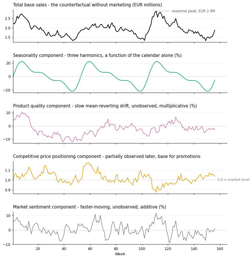
This is the counterfactual baseline the rest of the post builds on. The three firm-level factors move sales by broadly similar magnitudes — a few percent up or down in a typical week — but with very different dynamics. With the baseline in place, we can turn to the first layer of business activity: promotional pricing.
Step 2: Promotional Pricing
The promotional calendar is fixed and repeats every year: Cyber Week in late November, winter clearance in January, mid-season sales in spring and autumn, summer clearance in July. Major sales discount 40%, mid-season sales 30%.
Customer response depends on the occasion. Deal-hunting Cyber Week shoppers react more strongly to a 40% discount than customers in an ordinary week. I implement this by scaling the base price elasticity of −0.9 with an occasion-specific multiplier:
| Occasion | Discount | Multiplier | Resulting Price Elasticity |
|---|---|---|---|
| No promotion | - | 1.0 | −0.90 |
| Mid-season sale | 30% | 1.3 | −1.17 |
| Clearance | 40% | 1.5 | −1.35 |
| Cyber Week | 40% | 1.8 | −1.62 |
The sales multiplier in a promotion week is then \((1-d)^{\varepsilon}\), with \(d\) the discount and \(\varepsilon\) the occasion’s elasticity: a 40% discount in Cyber Week lifts sales by a factor of \(0.6^{-1.62} \approx 2.3\), the same discount in a clearance week by \(0.6^{-1.35} \approx 2.0\).
# The promotional calendar: fixed weeks within the year, fixed discount depths
PROMOTION_SCHEDULE = {
    'cyber_week':        {'weeks_in_year': [46, 47],  'discount': 0.4},
    'winter_clearance':  {'weeks_in_year': [2, 3, 4], 'discount': 0.4},
    'spring_mid_season': {'weeks_in_year': [16],      'discount': 0.3},
    'summer_clearance':  {'weeks_in_year': [28, 29],  'discount': 0.4},
    'autumn_mid_season': {'weeks_in_year': [40],      'discount': 0.3},
}

# Occasion-specific scaling of the base price elasticity
ELASTICITY_MULTIPLIERS = {
    'none': 1.0,
    'spring_mid_season': 1.3,
    'autumn_mid_season': 1.3,
    'winter_clearance': 1.5,
    'summer_clearance': 1.5,
    'cyber_week': 1.8,
}


def generate_promotional_calendar(n_weeks=156):
    """Roll the yearly schedule out over the full sample."""
    promotion_types = ['none'] * n_weeks
    true_discount_rates = np.zeros(n_weeks)
    for year_offset in range(0, n_weeks, 52):
        for promo_type, config in PROMOTION_SCHEDULE.items():
            for week in config['weeks_in_year']:
                t = year_offset + week
                if t < n_weeks:
                    promotion_types[t] = promo_type
                    true_discount_rates[t] = config['discount']
    return promotion_types, true_discount_rates
def calculate_true_promotional_effects(base_sales, base_price_level,
promotion_types, true_discount_rates):
"""
Apply occasion-dependent price elasticity to the promotional discounts.
Returns the true (error-free) promotional price level and sales uplift.
"""
n_weeks = len(base_sales)
# Promotional prices discount from the competitive price level of Step 1
true_promotional_price_level = base_price_level.copy()
for t in range(n_weeks):
if promotion_types[t] != 'none':
true_promotional_price_level[t] = (base_price_level[t]
* (1 - true_discount_rates[t]))
# Elasticity by week: base elasticity scaled by the occasion multiplier
true_elasticity_by_week = np.array([
BASE_PRICE_ELASTICITY * ELASTICITY_MULTIPLIERS[promo]
for promo in promotion_types
])
# Sales multiplier (1 - d)^elasticity, with guardrails that never bind here
price_ratio = np.maximum(1 - true_discount_rates, 0.5)
promotional_sales_multipliers = np.power(price_ratio, true_elasticity_by_week)
promotional_sales_multipliers = np.clip(promotional_sales_multipliers, 0.8, 3.0)
true_sales_with_promotions = base_sales * promotional_sales_multipliers
true_promotional_uplift = true_sales_with_promotions - base_sales
return {
'true_promotional_price_level': true_promotional_price_level,
'true_elasticity_by_week': true_elasticity_by_week,
'true_sales_with_promotions': true_sales_with_promotions,
'true_promotional_uplift': true_promotional_uplift
}Measurement error. Real promotional data is imperfect, and it is worth building the imperfection in rather than assuming it away. In practice, promotion periods sometimes get mislabelled; and pricing feeds carry errors that persist across weeks rather than averaging out. Two illustrative error processes mimic this: the observed promotion flag captures only 70% of true promotion weeks and adds false positives in 15% of ordinary weeks, and the observed price level carries autocorrelated noise with 20% persistence.
This creates a dual data structure that runs through the rest of the series: we have columns keeping track of the true promotional state, which we keep for grading, and the observed state, which is all the model will be given.
def generate_measurement_errors(true_promotional_price_level, promotion_types,
                                random_state=42):
    """
    The two data-quality problems of real promotional data:
    1. Promotion weeks are mislabelled (70% captured, 15% false positives)
    2. Observed prices carry sticky, autocorrelated errors (20% persistence)
    """
    np.random.seed(random_state)
    n_weeks = len(promotion_types)

    # Problem 1: the observed promotion flag
    observed_promotion_dummy = np.zeros(n_weeks)
    true_promo_indices = [i for i, p in enumerate(promotion_types) if p != 'none']
    if len(true_promo_indices) > 0:
        captured_count = int(len(true_promo_indices) * 0.70)
        captured = np.random.choice(true_promo_indices, captured_count, replace=False)
        observed_promotion_dummy[captured] = 1

    non_promo_indices = [i for i, p in enumerate(promotion_types) if p == 'none']
    if len(non_promo_indices) > 0:
        false_positive_count = int(len(non_promo_indices) * 0.15)
        false_positives = np.random.choice(non_promo_indices, false_positive_count,
                                           replace=False)
        observed_promotion_dummy[false_positives] = 1

    # Problem 2: sticky pricing errors
    pricing_noise = np.zeros(n_weeks)
    pricing_noise[0] = np.random.normal(0, 0.08)
    for t in range(1, n_weeks):
        pricing_noise[t] = 0.2 * pricing_noise[t - 1] + np.random.normal(0, 0.08)

    observed_promotional_price_level = true_promotional_price_level * (1 + pricing_noise)
    observed_promotional_price_level = np.clip(observed_promotional_price_level, 0.5, 1.8)

    return {
        'observed_promotion_dummy': observed_promotion_dummy,
        'observed_promotional_price_level': observed_promotional_price_level,
        'pricing_noise': pricing_noise
    }
Putting the pieces together:
promotion_types, true_discount_rates = generate_promotional_calendar(156)

true_promotion_effects = calculate_true_promotional_effects(
    base_data['base_sales'],
    base_data['base_price_level'],
    promotion_types,
    true_discount_rates
)

measured_promotion_effects = generate_measurement_errors(
    true_promotion_effects['true_promotional_price_level'],
    promotion_types
)

promotional_data_df = pd.DataFrame({
    'week': range(1, 157),
    'promotion_type': promotion_types,
    'true_discount_rate': true_discount_rates,
    'true_promotion_dummy': [1 if p != 'none' else 0 for p in promotion_types],
    'observed_promotion_dummy': measured_promotion_effects['observed_promotion_dummy'],
    'base_sales': base_data['base_sales'],
    'true_promotional_price_level': true_promotion_effects['true_promotional_price_level'],
    'true_sales_with_promotions': true_promotion_effects['true_sales_with_promotions'],
    'true_promotional_uplift': true_promotion_effects['true_promotional_uplift'],
    'observed_promotional_price_level': measured_promotion_effects['observed_promotional_price_level'],
})promotional_data_df.head(5)| week | promotion_type | true_discount_rate | true_promotion_dummy | observed_promotion_dummy | base_sales | true_promotional_price_level | true_sales_with_promotions | true_promotional_uplift | observed_promotional_price_level | |
|---|---|---|---|---|---|---|---|---|---|---|
| 0 | 1 | none | 0.0 | 0 | 0.0 | 2239.520824 | 1.000000 | 2239.520824 | 0.000000 | 0.957247 |
| 1 | 2 | none | 0.0 | 0 | 0.0 | 2203.448705 | 1.055973 | 2203.448705 | 0.000000 | 0.920645 |
| 2 | 3 | winter_clearance | 0.4 | 1 | 1.0 | 2320.906782 | 0.638755 | 4625.444876 | 2304.538094 | 0.582051 |
| 3 | 4 | winter_clearance | 0.4 | 1 | 1.0 | 2605.964209 | 0.613436 | 5193.549301 | 2587.585093 | 0.639042 |
| 4 | 5 | winter_clearance | 0.4 | 1 | 1.0 | 2489.169213 | 0.623910 | 4960.783030 | 2471.613818 | 0.618529 |
visualize_promotional_effects(promotional_data_df, show_summary=False)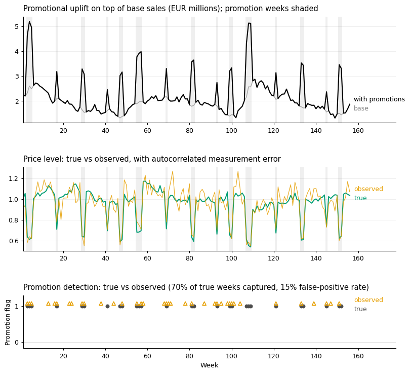
The promotional layer contributes three things the estimation will have to cope with: sharp, recurring sales spikes; customer response that varies by occasion; and observed promotion data that is wrong in realistic ways. None of these is exotic; they are the ordinary conditions under which the model will have to work. Next, marketing spend that coordinates around this calendar.
Step 3: Marketing Spend
Marketing spend in real companies is not random. It is the outcome of strategic planning, algorithmic optimisation, and budget cycles.
Strategic coordination. Marketing teams know the promotional calendar months in advance and ramp up spend two to three weeks before a sale to build awareness. Spend increases before sales-events, which creates a forward-looking correlation.
Algorithmic performance chasing. Bidding systems — Google product listing ads (PLA) in this data — monitor recent sales and adjust spend automatically: more when sales are strong, less when they are weak. Spend ends up correlated with sales through the optimisation loop, whether or not the spend caused anything.
Quarterly budget reviews. After a good quarter, the marketing budget grows; after a weak one, it is cut. A slow-moving correlation between past performance and future spend, unrelated to current effectiveness.
We model three marketing channels - television, Meta (Instagram and Facebook), and Google product listing ads (PLA). The channels combine these mechanisms differently, which is itself realistic. Meta follows the strategic calendar. TV adds concentrated bursts around Christmas and summer, planned long in advance and indifferent to weekly performance. PLA follows the calendar and chases performance. The implementation mirrors this structure: a planned component for every channel, and a performance-chasing multiplier applied on top for PLA.
Quarterly budget reviews
Every 13 weeks, the budget for the coming quarter is scaled by last quarter’s sales relative to the quarter before, with a sensitivity of 0.3 and bounds of -20% down, +40% up.
def generate_quarterly_budget_adjustments(sales_signal, sensitivity=0.3):
    """
    Quarterly budget reviews: each quarter's budget multiplier responds to
    the previous quarter's sales relative to the quarter before that.
    The first review with two full quarters of history is at week 26.
    """
    sales_signal = np.asarray(sales_signal)
    n_weeks = len(sales_signal)
    multipliers = np.ones(n_weeks)

    for quarter_start in range(26, n_weeks, 13):
        prev_quarter = sales_signal[quarter_start - 13:quarter_start].mean()
        quarter_before = sales_signal[quarter_start - 26:quarter_start - 13].mean()
        performance_ratio = prev_quarter / quarter_before
        adjustment = np.clip(1 + sensitivity * (performance_ratio - 1), 0.8, 1.4)
        multipliers[quarter_start:min(n_weeks, quarter_start + 13)] = adjustment

    return multipliers


sales_before_marketing = true_promotion_effects['true_sales_with_promotions']
quarterly_multipliers = generate_quarterly_budget_adjustments(sales_before_marketing)
One simplification: the reviews respond to sales before marketing effects, which keeps the data generation sequential. In reality budgets respond to total sales, marketing effects included. The coordination pattern that matters — budgets follow business performance with a quarterly lag — survives this simplification.
Planned spend
Planned spend for each channel starts from a base level and moves, in log space, with three terms: the quarterly budget multiplier, the seasonal planning cycle, and the number of promotion weeks coming up in the next three weeks — the strategic ramp-up. TV adds its bursts on top: 15× the base level in the five weeks before Christmas, 8× in early summer.
def count_upcoming_promotions(promotion_types, horizon=3):
    """For each week, the number of promotion weeks among the next `horizon` weeks."""
    n_weeks = len(promotion_types)
    is_promo = np.array([p != 'none' for p in promotion_types], dtype=int)
    upcoming = np.zeros(n_weeks, dtype=int)
    for t in range(n_weeks):
        upcoming[t] = is_promo[t + 1:min(n_weeks, t + 1 + horizon)].sum()
    return upcoming


# Base spend in thousands of euros; promo_coordination scales the pre-promotion
# ramp-up. TV coordinates through its planned bursts, not tactically.
CHANNEL_PLANNING = {
    'pla':  {'base_spend': 60, 'promo_coordination': 0.4},
    'meta': {'base_spend': 40, 'promo_coordination': 0.4},
    'tv':   {'base_spend': 10, 'promo_coordination': 0.0},
}

TV_BURSTS = {
    'christmas': {'weeks_in_year': range(47, 52), 'multiplier': 15},
    'summer':    {'weeks_in_year': range(20, 23), 'multiplier': 8},
}


def generate_planned_spend(n_weeks, seasonal_component, upcoming_promotions,
                           quarterly_multipliers, random_state=42):
    """
    The planned component of spend for every channel: base level, quarterly
    budget, seasonal planning, strategic ramp-up before promotions, and
    TV's burst calendar. All values in thousands of euros.
    """
    np.random.seed(random_state)
    seasonal_component = np.asarray(seasonal_component)
    spend_data = {}

    for channel, config in CHANNEL_PLANNING.items():
        spend = np.zeros(n_weeks)
        for t in range(n_weeks):
            log_spend = np.log(config['base_spend'])
            log_spend += np.log(quarterly_multipliers[t])
            log_spend += 0.15 * seasonal_component[t]
            log_spend += config['promo_coordination'] * upcoming_promotions[t]

            if channel == 'tv':
                week_in_year = t % 52
                for burst in TV_BURSTS.values():
                    if week_in_year in burst['weeks_in_year']:
                        log_spend += np.log(burst['multiplier'])

            log_spend += np.random.normal(0, 0.1)   # planning noise
            spend[t] = np.exp(log_spend)
        spend_data[channel] = spend

    return spend_data


upcoming_promotions = count_upcoming_promotions(promotion_types)
planned_spend = generate_planned_spend(
    156, base_data['seasonal_component'], upcoming_promotions, quarterly_multipliers
)
Performance chasing
The algorithmic component deserves the most care, because it produces the endogeneity that later proves hardest to remove.
Modern bidding systems adjust spend continuously in response to results. The stylised version here: each week, the algorithm compares recent sales — with a one-week reporting lag — against its own baseline, a ten-week rolling average, and scales spend up or down in proportion to the gap, within bounds. When sales are above the recent average, PLA spend rises; when they are below, it falls.
The attribution problem follows directly. When PLA spend is high during a sales spike, there are two candidate explanations: the spend caused the spike, or the algorithm detected the spike and moved to capture it. In the data both look identical — spend and sales moving together — and a Marketing Mix Model has no way to tell them apart from the time series alone. Strategic coordination at least follows a calendar, which a model can control for. The algorithm responds to realised performance, including its random component, and no function of the calendar can proxy for that.
One simplification (similar to the one for modelling budget reviews): the algorithm here observes sales before marketing effects. In reality it would observe total sales, its own contribution included — a feedback loop. Modelling the loop would require simulating week by week; I keep the causal structure acyclic instead, at the cost of understating PLA’s endogeneity somewhat. The essential mechanism — spend follows performance signals — is preserved.
def performance_chasing_multipliers(sales_signal, sensitivity=0.8,
                                    response_lag=1, baseline_window=10,
                                    bounds=(0.5, 3.0)):
    """
    The bidding algorithm as a weekly spend multiplier: recent sales
    (with a reporting lag) relative to a rolling baseline, scaled by the
    algorithm's sensitivity and clipped to its safety bounds.
    Deterministic given the sales signal.
    """
    sales_signal = np.asarray(sales_signal)
    n_weeks = len(sales_signal)
    multipliers = np.ones(n_weeks)

    for t in range(baseline_window + response_lag, n_weeks):
        recent = sales_signal[t - response_lag:t].mean()
        baseline = sales_signal[t - baseline_window - response_lag:t - response_lag].mean()
        performance_ratio = recent / baseline
        multipliers[t] = np.clip(1 + sensitivity * (performance_ratio - 1),
                                 bounds[0], bounds[1])

    return multipliers


chasing_multipliers = performance_chasing_multipliers(sales_before_marketing)

# Final spend: the planned series for every channel, with the chasing
# multiplier applied on top for PLA only
marketing_spend = dict(planned_spend)
marketing_spend['pla'] = planned_spend['pla'] * chasing_multipliers
visualize_marketing_spend_patterns(marketing_spend, planned_spend['pla'],
promotion_types, base_data,
true_promotion_effects, quarterly_multipliers,
show_summary=False)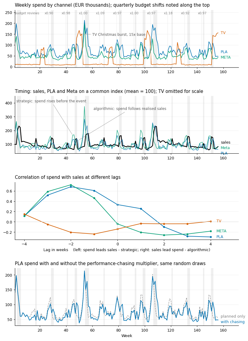
The third panel compresses the endogeneity into one picture. At negative lags, the correlation measures how well spend predicts future sales; at positive lags, how well past sales predict spend. Both PLA and Meta correlate strongly at negative lags — the strategic ramp-up ahead of promotions, which the two channels share. The difference sits on the right-hand side: once sales lead spend, Meta’s correlation falls away, while PLA’s stays positive — the signature of an algorithm following realised performance. TV shows little of either; its bursts follow the calendar, not the sales signal. The fourth panel isolates the algorithmic component directly — the same PLA series with and without the chasing multiplier, on identical random draws.
None of this coordination is noise to be cleaned away. It is how a competent retailer operates, and a synthetic benchmark that omitted it would flatter the model. What remains is the final layer: converting this spend into the sales effects the model will later try to recover.
Step 4: Marketing Effects
Spend becomes sales through the two transformations that Marketing Mix Models assume: adstock for carryover, saturation for diminishing returns. Because the goal is to test whether an MMM can recover known effects, the data uses exactly the transformations the model will later fit. This is a deliberate gift to the model — whatever goes wrong in estimation cannot be blamed on functional form.
The two functions below reappear in identical form throughout the series: the estimation notebook implements the same equations inside PyMC, and the calibration notebook uses these definitions directly.
Adstock: carryover over time
Advertising this week does not only translate into additional sales this week. The ad lingers on people’s minds, or people simply take time to purchase after seeing it. This delayed effect is called carryover or adstock: each week’s spend is spread over the current and following weeks with geometrically decaying weights — with a retention rate of 70%, each week carries 70% of the previous week’s share, truncated here at six weeks.
It is convention to normalise the weights to sum to one, so adstock redistributes spend over time without changing its total: total exposure equals total spend, which keeps the coefficients — and later the ROAS figures — interpretable. One consequence is worth stating explicitly, because it trips up the intuition: with 70% retention, a given week does not carry the full effect of the spend in that week, but only about a third of it (34%), the next week 24%, the week after 17%, and so on. The 70% describes the decay between weeks, not the share of the first one.
def geometric_adstock(spend_series, adstock_rate, l_max=6):
    """
    Geometric carryover with weights normalised to sum to one, so total
    exposure equals total spend. Weeks before the sample are treated as zero.
    """
    weights = adstock_rate ** np.arange(l_max)
    weights = weights / weights.sum()
return np.convolve(spend_series, weights)[:len(spend_series)]visualize_adstock_weights(rates=(0.2, 0.4, 0.7))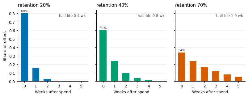
Saturation: diminishing returns
When spending on marketing, the second EUR 100K might buy you less than the first EUR 100K: the most receptive customers have already been reached. We model this through logistic saturation, \(\frac{1-e^{-\lambda x}}{1+e^{-\lambda x}}\), which maps adstocked spend into \([0,1)\): it rises steeply at first and flattens toward a ceiling of 1. The parameter \(\lambda\) controls how quickly the ceiling is approached, but it has no intuitive units on its own. A more readable quantity is the half-saturation spend — the spend at which a channel delivers half of its maximum possible effect. Setting the expression equal to \(\tfrac{1}{2}\) and solving gives \(x_{1/2} = \ln 3/ \lambda\). For the flattest of the three curves below, \(\lambda = 0.006\), that is about EUR 183K: at that level of (adstocked) spend, the channel has exhausted half of what it can ever contribute per week.
def logistic_saturation(adstocked_series, lam):
    """Diminishing returns. Spend is in thousands of euros; no further scaling."""
    return (1 - np.exp(-lam * adstocked_series)) / (1 + np.exp(-lam * adstocked_series))
visualize_saturation_curves(logistic_saturation, lambdas=(0.008, 0.01, 0.006))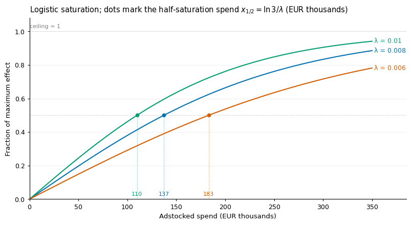
Channel parameters
The channels differ in carryover and saturation according to their role. PLA: 20% carryover — performance marketing acts quickly — with half-saturation near EUR 137K and a coefficient set for roughly 4× ROAS. Meta: 40% carryover, mixed brand and performance marketing, half-saturation near EUR 110K, roughly 3× ROAS. TV: 70% carryover — brand building — the flattest curve with half-saturation near EUR 183K, roughly 1.5× ROAS. The ROAS levels are illustrative, in the range of published industry benchmarks.
# All monetary values in thousands of euros.
CHANNEL_CONFIGS = {
    'pla': {
        'adstock_rate': 0.2,         # fast decay: performance marketing acts now
        'saturation_lambda': 0.008,  # half-saturation at ln(3)/0.008 = EUR 137K
        'coefficient': 1100          # gives roughly 4x ROAS
    },
    'meta': {
        'adstock_rate': 0.4,         # mixed brand / performance
        'saturation_lambda': 0.01,   # half-saturation at EUR 110K
        'coefficient': 600           # roughly 3x ROAS
    },
    'tv': {
        'adstock_rate': 0.7,         # long brand-building carryover
        'saturation_lambda': 0.006,  # flattest curve: half-saturation at EUR 183K
        'coefficient': 560           # roughly 1.5x ROAS
    }
}
The three retention rates and three saturation curves above are, in fact, the three channels.
A note on units, looking ahead. This notebook works in unscaled thousands of euros, so \(\lambda\) is numerically small (0.006–0.010 per EUR K). The estimation notebook will divide every series by its maximum before sampling. The parameters \(\lambda\) and \(\beta\) are not scale-invariant - hence it matters whether we estimate a model with spends expressed in EUR, spends in thousands of EUR, or spends scaled in other ways: the parameters only mean something relative to the scale of the data. Keeping this in mind avoids the most common confusion when comparing estimates against the ground truth.
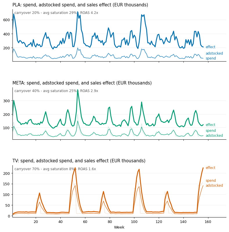
The pipeline per channel is spend → adstock → saturation → coefficient. The function records the intermediate series as well; they feed the figure and the validation printout.
def apply_marketing_transformations(spend_data):
    """Convert spend into sales effects: adstock, then saturation, then scale."""
    marketing_effects = {}
    total_marketing_uplift = 0
    transformation_details = {}

    for channel, spend in spend_data.items():
        config = CHANNEL_CONFIGS[channel]

        adstocked = geometric_adstock(spend, config['adstock_rate'])
        saturated = logistic_saturation(adstocked, config['saturation_lambda'])
        marketing_effects[channel] = config['coefficient'] * saturated
        total_marketing_uplift += marketing_effects[channel]

        transformation_details[channel] = {
            'avg_spend': spend.mean(),
            'avg_adstocked': adstocked.mean(),
            'avg_saturation': saturated.mean(),
            'avg_effect': marketing_effects[channel].mean(),
            'implied_roas': (marketing_effects[channel].mean() / spend.mean()
                             if spend.mean() > 0 else 0),
            'adstocked': adstocked,
            'saturated': saturated,
        }

    return marketing_effects, total_marketing_uplift, transformation_details
marketing_effects, total_marketing_uplift, transformation_details = \
apply_marketing_transformations(marketing_spend)
adstocked = {ch: d['adstocked'] for ch, d in transformation_details.items()}
saturated = {ch: d['saturated'] for ch, d in transformation_details.items()}
visualize_marketing_transformations(
marketing_spend=marketing_spend,
adstocked_spend=adstocked,
saturated_spend=saturated,
marketing_effects=marketing_effects,
transformation_details=transformation_details,
CHANNEL_CONFIGS=CHANNEL_CONFIGS,
show_details=True,
n_weeks=156
)
TRANSFORMATION CHECKS
==================================================

PLA:
  average spend           EUR 76K per week
  half-saturation spend   EUR 137K (spend at which the curve reaches 50%)
  implied ROAS            4.2x
  saturation at spend of EUR 50K: 20%   EUR 100K: 38%   EUR 150K: 54%   EUR 200K: 66%

META:
  average spend           EUR 53K per week
  half-saturation spend   EUR 110K (spend at which the curve reaches 50%)
  implied ROAS            2.9x
  saturation at spend of EUR 50K: 24%   EUR 100K: 46%   EUR 150K: 64%   EUR 200K: 76%

TV:
  average spend           EUR 28K per week
  half-saturation spend   EUR 183K (spend at which the curve reaches 50%)
  implied ROAS            1.6x
  saturation at spend of EUR 50K: 15%   EUR 100K: 29%   EUR 150K: 42%   EUR 200K: 54%
Each channel’s effect now follows the model’s own assumptions: carryover that preserves total impact, diminishing returns at plausible spend levels, and ROAS in a realistic range.
Step 5: The Complete Dataset
The four layers combine additively:
\[\text{total sales}_t \;=\; \text{base}_t \;+\; \text{promotional uplift}_t \;+\; \sum_{c} \text{marketing effect}_{c,t}\]
The assembled table carries the dual structure introduced in Step 2, now for everything. The observed columns are what an analyst would receive: total sales, spend per channel, the noisy promotion flag and price level. The ground-truth columns are what we keep for grading: the decomposition of every euro of sales, the true promotional state, each channel’s true effect. The estimator will be fit on the former; the latter exist to evaluate it.
def assemble_final_dataset(base_data, promotional_data_df, marketing_spend,
                           marketing_effects):
    """
    The complete dataset. Causal flow:
    base_sales + promotional_uplift + marketing_uplift = total_sales
    """
    n_weeks = len(base_data)

    total_sales = (base_data['base_sales'] +
                   promotional_data_df['true_promotional_uplift'] +
                   sum(marketing_effects.values()))

    dataset = pd.DataFrame({
        # Time
        'week': range(1, n_weeks + 1),
        'year': [(w - 1) // 52 + 1 for w in range(1, n_weeks + 1)],
        'week_of_year': [(w - 1) % 52 + 1 for w in range(1, n_weeks + 1)],

        # Outcome and its true decomposition
        'total_sales': total_sales,
        'base_sales': base_data['base_sales'],
        'promotional_sales_uplift': promotional_data_df['true_promotional_uplift'],
        'marketing_sales_uplift': sum(marketing_effects.values()),

        # Base components (unobserved in real data)
        'seasonal_component': base_data['seasonal_component'],
        'quality_factor': base_data['quality_factor'],
        'base_price_level': base_data['base_price_level'],
        'market_sentiment': base_data['market_sentiment'],

        # Promotions: true state (for grading)
        'promotion_type': promotional_data_df['promotion_type'],
        'true_discount_rate': promotional_data_df['true_discount_rate'],
        'true_promotion_dummy': promotional_data_df['true_promotion_dummy'],
        'true_promotional_price_level': promotional_data_df['true_promotional_price_level'],

        # Promotions: observed state (what the model sees)
        'observed_promotion_dummy': promotional_data_df['observed_promotion_dummy'],
        'observed_promotional_price_level': promotional_data_df['observed_promotional_price_level'],

        # Marketing spend (what the model sees)
        'pla_spend': marketing_spend['pla'],
        'meta_spend': marketing_spend['meta'],
        'tv_spend': marketing_spend['tv'],

        # Marketing effects (for grading)
        'pla_effect': marketing_effects['pla'],
        'meta_effect': marketing_effects['meta'],
        'tv_effect': marketing_effects['tv'],
        'total_marketing_effect': sum(marketing_effects.values())
    })

    return dataset


synthetic_dataset = assemble_final_dataset(
    base_data=base_data,
    promotional_data_df=promotional_data_df,
    marketing_spend=marketing_spend,
    marketing_effects=marketing_effects
)synthetic_dataset.head(5)| week | year | week_of_year | total_sales | base_sales | promotional_sales_uplift | marketing_sales_uplift | seasonal_component | quality_factor | base_price_level | ... | true_promotional_price_level | observed_promotion_dummy | observed_promotional_price_level | pla_spend | meta_spend | tv_spend | pla_effect | meta_effect | tv_effect | total_marketing_effect | |
|---|---|---|---|---|---|---|---|---|---|---|---|---|---|---|---|---|---|---|---|---|---|
| 0 | 1 | 1 | 1 | 2896.414275 | 2239.520824 | 0.000000 | 656.893451 | 0.000000 | 0.049671 | 1.000000 | ... | 1.000000 | 0.0 | 0.957247 | 140.332692 | 107.281573 | 10.860439 | 463.268805 | 187.421404 | 6.203243 | 656.893451 |
| 1 | 2 | 1 | 2 | 3196.504325 | 2203.448705 | 0.000000 | 993.055621 | 0.054956 | 0.044423 | 1.055973 | ... | 1.055973 | 0.0 | 0.920645 | 198.097935 | 140.401496 | 10.937305 | 681.164797 | 301.302236 | 10.588588 | 993.055621 |
| 2 | 3 | 1 | 3 | 5495.854098 | 2320.906782 | 2304.538094 | 870.409222 | 0.106231 | 0.055155 | 1.064591 | ... | 0.638755 | 1.0 | 0.582051 | 144.755790 | 80.293109 | 11.577548 | 596.991585 | 259.394564 | 14.023073 | 870.409222 |
| 3 | 4 | 1 | 4 | 5903.182328 | 2605.964209 | 2587.585093 | 709.633027 | 0.150513 | 0.082858 | 1.022393 | ... | 0.613436 | 1.0 | 0.639042 | 106.615036 | 65.177337 | 10.249844 | 475.591387 | 218.372803 | 15.668836 | 709.633027 |
| 4 | 5 | 1 | 5 | 5439.086606 | 2489.169213 | 2471.613818 | 478.303576 | 0.185183 | 0.074032 | 1.039850 | ... | 0.623910 | 1.0 | 0.618529 | 60.262295 | 37.307287 | 11.007290 | 305.694983 | 155.355628 | 17.252965 | 478.303576 |
5 rows × 24 columns
visualize_complete_dataset(synthetic_dataset, show_summary=True)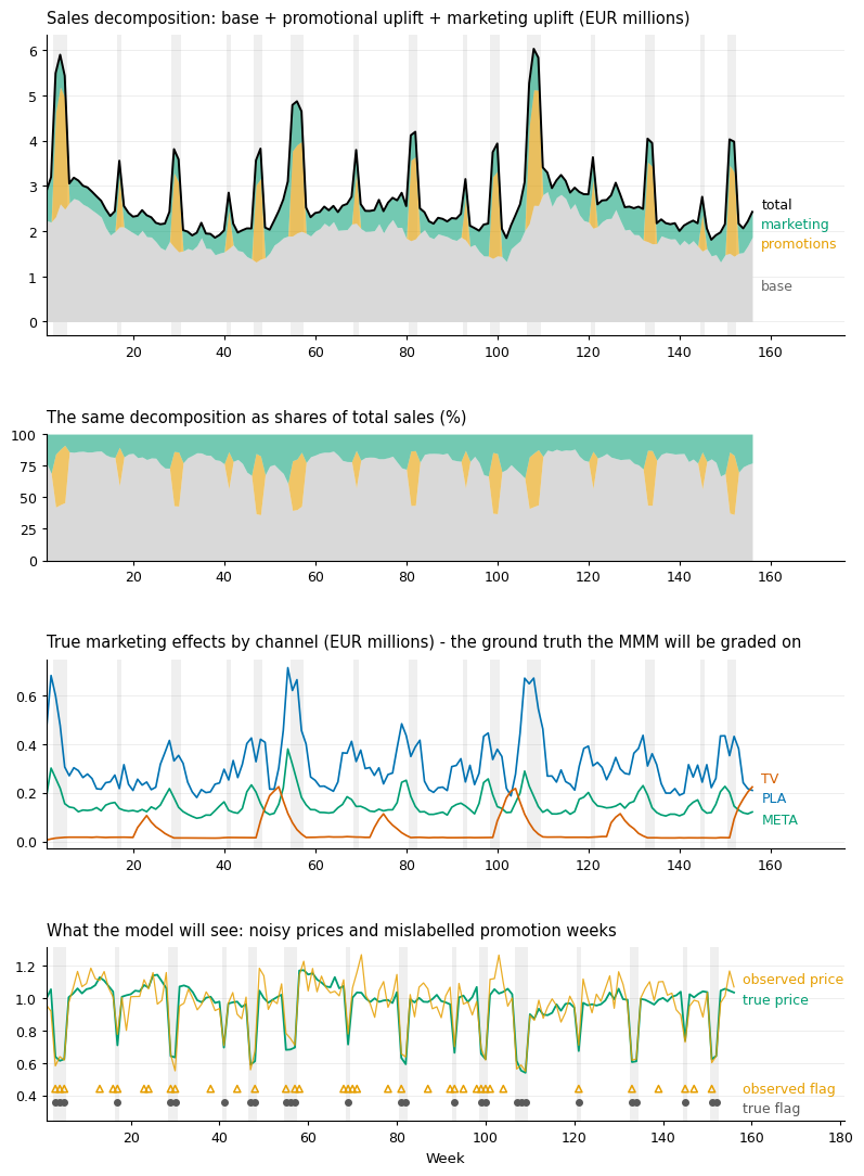
COMPLETE DATASET SUMMARY
==================================================
Shape: 156 weeks (3.0 years), 24 columns
Total sales: EUR 1,812K to EUR 6,035K per week

Decomposition of cumulative sales:
  base sales           70.3%
  promotional uplift   11.1%
  marketing uplift     18.7%

True ROAS by channel:
  PLA   4.20x
  META  2.90x
  TV    1.56x

Promotion detection accuracy: 82.1%
Price measurement correlation: 0.891synthetic_dataset.to_csv("synthetic_mmm_data.csv", index=False)Conclusion
The dataset now carries the complexity that a Marketing Mix Model will realistically have to deal with: seasonality, sales and discounts - and consumers responding to them, marketing spend shaped by planning and by algorithms, and smaller measurement errors — together with an exact record of the truth underneath.
The simplifications are worth listing. There are no competitive responses, no supply-chain constraints forcing promotional timing, no other shocks to demand. The bidding algorithm is stylised — real systems use richer signals than recent sales — and it deliberately does not see its own effects, which understates the feedback problem rather than overstating it. These choices keep the causal structure tractable while retaining the coordination patterns that matter most.
In the next post, we build a Bayesian Marketing Mix Model from scratch, fit it to this data, and grade it against the truth we have just buried in it.
References
Jin, Y., Wang, Y., Sun, Y., Chan, D., & Koehler, J. (2017). Bayesian Methods for Media Mix Modeling with Carryover and Shape Effects. Google Inc.
Runge, J., Skokan, I., Zhou, G., & Pauwels, K. (2025). Packaging Up Media Mix Modeling: An Introduction to Robyn. arXiv:2403.14674.
Meta Marketing Science (2024). Robyn: Open Source Marketing Mix Modeling. GitHub repository: https://github.com/facebookexperimental/Robyn
Nguyen, J. (2022). siMMMulator: An Open-Source R Package to Generate Simulated Data for Marketing Mix Models. Meta. https://facebookexperimental.github.io/siMMMulator/
Vaver, J., & Zhang, S. (2017). Introduction to the Aggregate Marketing System Simulator. Google Inc.
PyMC Labs (2024). PyMC-Marketing: Open Source Marketing Analytics Solution. https://www.pymc-marketing.io/
Google (2025). Meridian: Marketing Mix Modeling Framework. https://developers.google.com/meridian
Note: All data, parameters, and business patterns in this post are fictional and do not reflect any specific company’s operations, performance metrics, or proprietary information. Parameter values were chosen by Claude, based on publicly available knowledge and the academic literature.